
Full resolution (JPEG) - On this page / på denna sida - Transducer Properties in Magnetostrictive Delay Lines, ny Gunnar Svala
<< prev. page << föreg. sida << >> nästa sida >> next page >>
Below is the raw OCR text
from the above scanned image.
Do you see an error? Proofread the page now!
Här nedan syns maskintolkade texten från faksimilbilden ovan.
Ser du något fel? Korrekturläs sidan nu!
This page has never been proofread. / Denna sida har aldrig korrekturlästs.
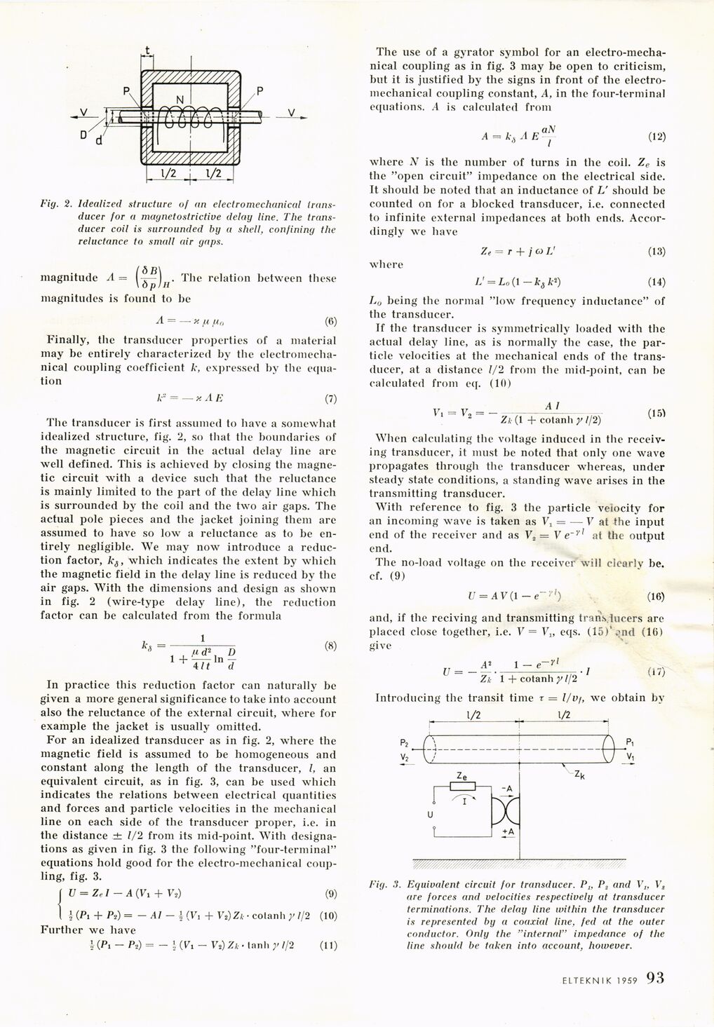
Fig. 2. Idealized structure of an electromechanical
transducer for a magnetostrictive delay line. The
transducer coil is surrounded by a shell, confining the
reluctance to small air gaps.
relation between these
magnitude A = . The
ö \ d p IH
magnitudes is found to be
A = — * fi /un (6)
Finally, the transducer properties of a material
may be entirely characterized by the
electromechanical coupling coefficient k, expressed by the
equation
k- = —xAE (7)
The transducer is first assumed to have a somewhat
idealized structure, fig. 2, so that the boundaries of
the magnetic circuit in the actual delay line are
well defined. This is achieved by closing the
magnetic circuit with a device such that the reluctance
is mainly limited to the part of the delay line which
is surrounded by the coil and the two air gaps. The
actual pole pieces and the jacket joining them are
assumed to have so low a reluctance as to be
entirely negligible. We may now introduce a
reduction factor, ks, which indicates the extent by which
the magnetic field in the delay line is reduced by the
air gaps. With the dimensions and design as showrn
in fig. 2 (wire-type delay line), the reduction
factor can be calculated from the formula
kx =
, , V d* D
477 tf
(8)
In practice this reduction factor can naturally be
given a more general significance to take into account
also the reluctance of the external circuit, where for
example the jacket is usually omitted.
For an idealized transducer as in fig. 2, where the
magnetic field is assumed to be homogeneous and
constant along the length of the transducer, I, an
equivalent circuit, as in fig. 3, can be used which
indicates the relations between electrical quantities
and forces and particle velocities in the mechanical
line on each side of the transducer proper, i.e. in
the distance ± 1/2 from its mid-point. With
designations as given in fig. 3 the following "four-terminal"
equations hold good for the electro-mechanical
coupling, fig. 3.
j U = Ze I — A (Vi + V-2) (9)
1 \ (Pi + P-j) = -Al -\(V, + Vi)Zk • cotanh y 1/2 (10)
Further we have
I (Pl - P-j) = - }, (Vi - Vs) Zk • tanh y 1/2 (11)
The use of a gyrator symbol for an
electro-mechanical coupling as in fig. 3 may be open to criticism,
but it is justified by the signs in front of the
electromechanical coupling constant, A, in the four-terminal
equations. .4 is calculated from
A = k\ A E
aN
I
(12)
where A7 is the number of turns in the coil. Ze is
the "open circuit" impedance on the electrical side.
It should be noted that an inductance of L’ should be
counted on for a blocked transducer, i.e. connected
to infinite external impedances at both ends.
Accordingly we have
Ze=r + jG)U (13)
where
/,’ = Lo (1 -ks A-2) (14)
Lo being the normal "low frequency inductance" of
the transducer.
Tf the transducer is symmetrically loaded with the
actual delay line, as is normally the case, the
particle velocities at the mechanical ends of the
transducer, at a distance 1/2 from the mid-point, can be
calculated from eq. (10)
A 1
V2 Zk (1 + cotanh >> 1/2)
When calculating the voltage induced in the
receiving transducer, it must be noted that only one wave
propagates through the transducer whereas, under
steady state conditions, a standing wave arises in the
transmitting transducer.
With reference to fig. 3 the particle velocity for
an incoming wave is taken as Vt — — V at the input
end of the receiver and as V2= V e~r’ at the output
end.
The no-load voltage on the receiver will clcarlv be.
cf. (9)
U = AV(l -e~’’) (16)
and, if the reciving and transmitting transducers are
placed close together, i.e. V = Vlt eqs. (15)’ ond (16)
U = -
A2
1 - e-i"
/
(17)
Zk 1 + cotanh y 1/2
Introducing the transit time r = l/vf, we obtain by
1/2 ^ 1/2
Fig. 3. Equivalent circuit for transducer. P„ Ps and Vj, Vt
are forces and velocities respectively at transducer
terminations. The delay line within the transducer
is represented by a coaxial line, fed at the outer
conductor. O nig the "internal" impedance of the
line should be taken into account, however.
ELTEKNIK 1959 1 93
<< prev. page << föreg. sida << >> nästa sida >> next page >>