
Full resolution (JPEG) - On this page / på denna sida - Transducer Properties in Magnetostrictive Delay Lines, ny Gunnar Svala
<< prev. page << föreg. sida << >> nästa sida >> next page >>
Below is the raw OCR text
from the above scanned image.
Do you see an error? Proofread the page now!
Här nedan syns maskintolkade texten från faksimilbilden ovan.
Ser du något fel? Korrekturläs sidan nu!
This page has never been proofread. / Denna sida har aldrig korrekturlästs.
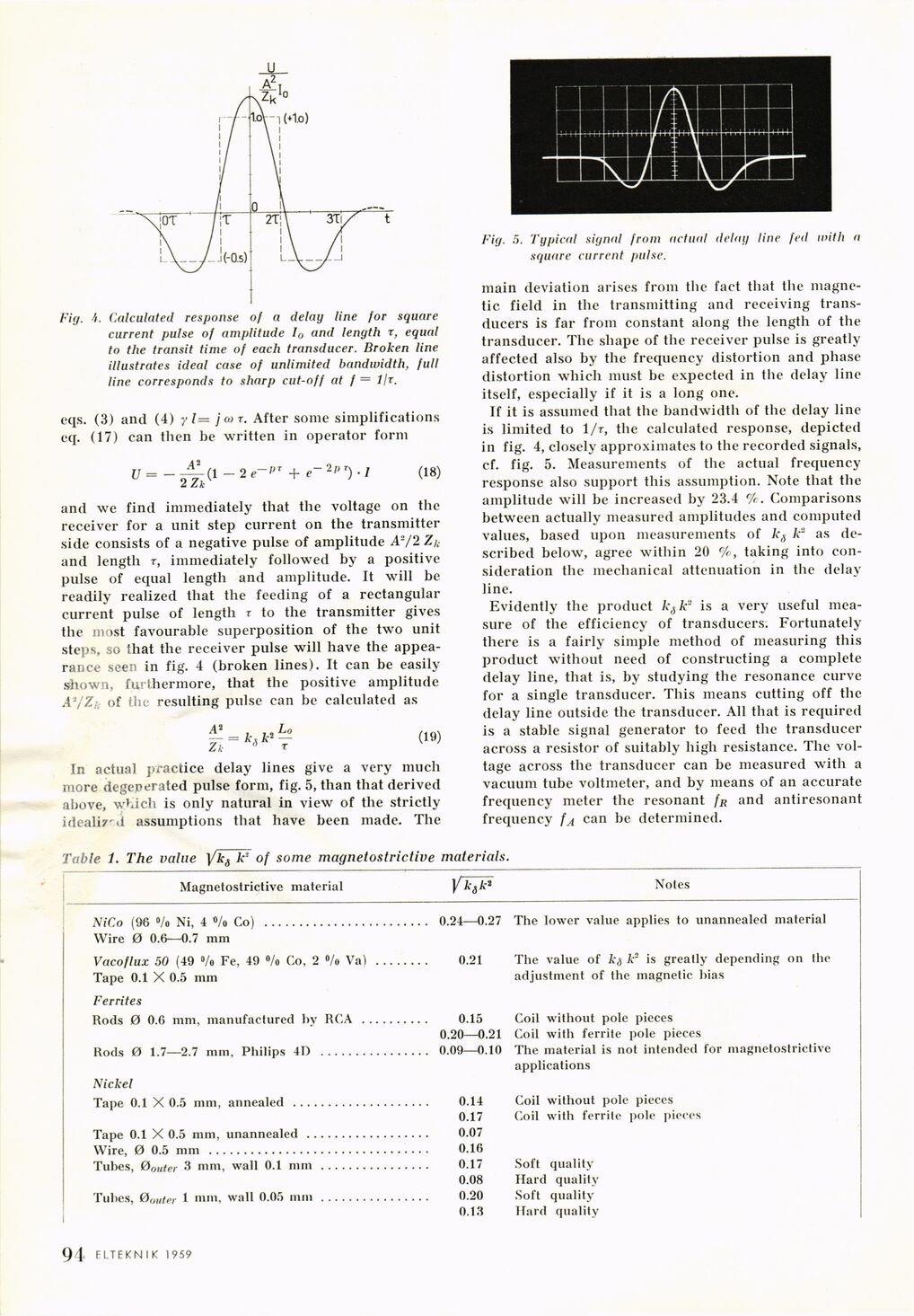
Fig. Calculated response of a delay line for square
current pulse of amplitude I0 ond length r, equal
to the transit time of each transducer. Broken line
illustrates ideal case of unlimited bandwidth, full
line corresponds to sharp cut-off at f — lit.
eqs. (3) and (4) yl= jcor. After some simplifications
eq. (17) can then he written in operator form
U = " 2T*(1 ~ 2 + 2P T) ’ 7 (18)
and we find immediately that the voltage on the
receiver for a unit step current on the transmitter
side consists of a negative pulse of amplitude A2/2 Z/{
and length r, immediately followed by a positive
pulse of equal length and amplitude. It will be
readily realized that the feeding of a rectangular
current pulse of length r to the transmitter gives
the most favourable superposition of the two unit
steps, so that the receiver pulse will have the
appearance seen in fig. 4 (broken lines). It can be easily
shown, furthermore, that the positive amplitude
A1 j7.1 of the resulting pulse can be calculated as
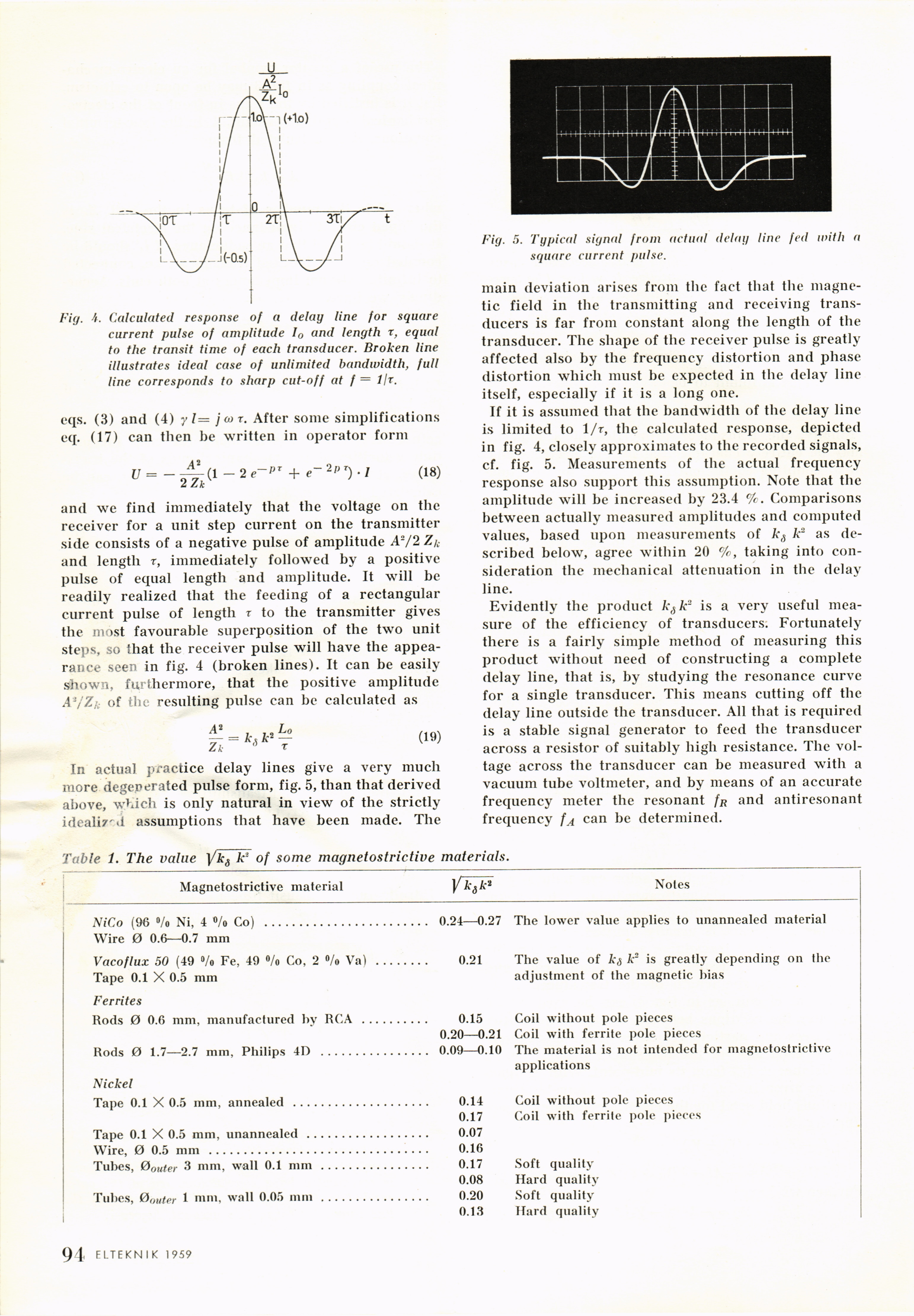
In actual practice delay lines give a very much
more degenerated pulse form, fig. 5, than that derived
above, which is only natural in view of the strictly
idealized assumptions that have been made. The
Fig. 5. Typical signal from actual delay line fed with a
square current pulse.
main deviation arises from the fact that the
magnetic field in the transmitting and receiving
transducers is far from constant along the length of the
transducer. The shape of the receiver pulse is greatly
affected also by the frequency distortion and phase
distortion which must be expected in the delay line
itself, especially if it is a long one.
If it is assumed that the bandwidth of the delay line
is limited to 1/r, the calculated response, depicted
in fig. 4, closely approximates to the recorded signals,
cf. fig. 5. Measurements of the actual frequency
response also support this assumption. Note that the
amplitude will be increased by 23.4 %. Comparisons
between actually measured amplitudes and computed
values, based upon measurements of ks k2 as
described below, agree within 20 taking into
consideration the mechanical attenuation in the delay
line.
Evidently the product ksk2 is a very useful
measure of the efficiency of transducers. Fortunately
there is a fairly simple method of measuring this
product without need of constructing a complete
delay line, that is, by studying the resonance curve
for a single transducer. This means cutting off the
delay line outside the transducer. All that is required
is a stable signal generator to feed the transducer
across a resistor of suitably high resistance. The
voltage across the transducer can be measured with a
vacuum tube voltmeter, and by means of an accurate
frequency meter the resonant /r and antiresonant
frequency can be determined.
Table i. The value Ykö k1 of some magnetostrictive materials.
Magnetostrictive material Vk6k* Notes
NiCo (96 °/o Ni, 4 °/o Co) .................... Wire 0 0.6—0.7 mm 0.24—0.27 The lower value applies to unannealed material
Vacoflux 50 (49 %> Fe, 49 °/o Co, 2 %> Va) Tape 0.1 X 0.5 mm 0.21 The value of k,5 k2 is greatly depending on the adjustment of the magnetic bias
Ferrites
Rods 0 0.6 mm, manufactured bv RCA ...... ____ 0.15 Coil without pole pieces
0.20—0.21 Coil with ferrite pole pieces
Rods 0 1.7—2.7 mm, Philips 4D ............ 0.09—0.10 The material is not intended for magnetostrictive applications
Nickel
Tape 0.1 X 0.5 mm, annealed ................ 0.14 Coil without pole pieces
0.17 Coil with ferrite pole pieces
Tape 0.1 X 0.5 mm, unannealed .............. ____ 0.07
Wire, 0 0.5 mm ............................ ____ 0.16
Tubes, Øouter 3 mm, wall 0.1 mm ............ ____ 0.17 Soft quality
0.08 Hard quality
Tubes, Øonter 1 mm, wall 0.05 mm............ 0.20 Soft quality
0.13 Hard quality
] 94 ELTEKN I K 1959
<< prev. page << föreg. sida << >> nästa sida >> next page >>